 Qww – wastewater discharge (calculated flow)
K – discharge coefficient
DU – connection value of unit
Qtot – total wastewater discharge
Qs – continous wastewater discharge (without simultaneity reduction)
From the sum DU, the wastewater discharge Qww can be calculated with the above formula, taking into account the corresponding discharge coefficient K. If the determined wastewater discharge Qww is smaller than the largest connected value of a single drainage object, the latter is decisive (limit value).
Qww – wastewater discharge (calculated flow)
K – discharge coefficient
DU – connection value of unit
Qtot – total wastewater discharge
Qs – continous wastewater discharge (without simultaneity reduction)
From the sum DU, the wastewater discharge Qww can be calculated with the above formula, taking into account the corresponding discharge coefficient K. If the determined wastewater discharge Qww is smaller than the largest connected value of a single drainage object, the latter is decisive (limit value). Waste water drainage
The wastewater discharge Qww according to DIN EN 12056-2, is determined from the sum of the connected loads (DU), taking into account the simultaneity, where K is the guide value for the discharge coefficient. It depends on the type of building and results from the frequency of use of the drainage objects.
Qww – wastewater discharge (calculated flow)
K – discharge coefficient
DU – connection value of unit
Qtot – total wastewater discharge
Qs – continous wastewater discharge (without simultaneity reduction)
From the sum DU, the wastewater discharge Qww can be calculated with the above formula, taking into account the corresponding discharge coefficient K. If the determined wastewater discharge Qww is smaller than the largest connected value of a single drainage object, the latter is decisive (limit value).
Qww – wastewater discharge (calculated flow)
K – discharge coefficient
DU – connection value of unit
Qtot – total wastewater discharge
Qs – continous wastewater discharge (without simultaneity reduction)
From the sum DU, the wastewater discharge Qww can be calculated with the above formula, taking into account the corresponding discharge coefficient K. If the determined wastewater discharge Qww is smaller than the largest connected value of a single drainage object, the latter is decisive (limit value).  Qs – Rainwater drainage (calculated flow)
rT(n) – Dimensioning value according to statistical events
C – Characteristic coefficient for type of drainage area
A – Size of drainage area
Qs – Rainwater drainage (calculated flow)
rT(n) – Dimensioning value according to statistical events
C – Characteristic coefficient for type of drainage area
A – Size of drainage area 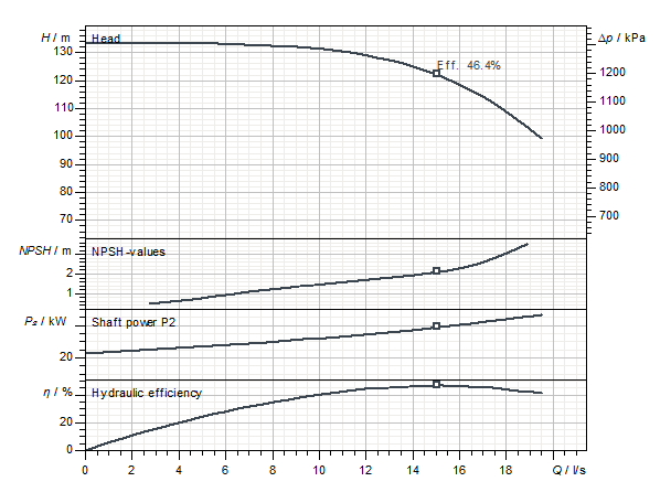
 In addition to the Q-H performance curve, the following performance curves are often found for centrifugal pumps:
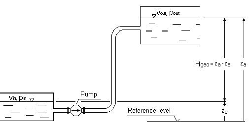
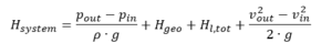 pin, pout = pressures on suction respectively discharge liquid levels
ρ = fluid density
g = gravity (9.81 m/s2)
Hgeo = static height difference between suction and discharge liquid levels
Hl,tot = total pipe friction loss between inlet and outlet areas
vin, vout = mean flow velocities at inlet and outlet liquid level areas
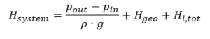
The mean flow velocities at the inlet and outlet areas are, based on the Continuity Law, mostly insignificantly small and can be neglected, if the tank areas being relatively large compared to those of the pipe work. In this case, above formula will be simplified to:
pin, pout = pressures on suction respectively discharge liquid levels
ρ = fluid density
g = gravity (9.81 m/s2)
Hgeo = static height difference between suction and discharge liquid levels
Hl,tot = total pipe friction loss between inlet and outlet areas
vin, vout = mean flow velocities at inlet and outlet liquid level areas
The mean flow velocities at the inlet and outlet areas are, based on the Continuity Law, mostly insignificantly small and can be neglected, if the tank areas being relatively large compared to those of the pipe work. In this case, above formula will be simplified to:
 The static portion of the system H-Q curve, that part that is unrelated to the rate of flow, reads:
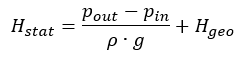 For closed circulating systems this value becomes zero.
The total friction losses are the sum of the frictional losses of all components in the suction and delivery piping. They vary, at sufficiently large REYNOLDS numbers, as the square of the flow rate.
For closed circulating systems this value becomes zero.
The total friction losses are the sum of the frictional losses of all components in the suction and delivery piping. They vary, at sufficiently large REYNOLDS numbers, as the square of the flow rate.
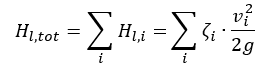
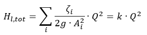 g = gravity (9.81 m/s2)
Hl,tot = total friction loss between inlet and outlet areas
vi = mean flow velocities trough pipe cross-section area
Ai = characteristic pipe cross-sectional area
ζi = friction loss coefficient for pipes, fittings, etc.
Q = flow rate
k = proportionality factor
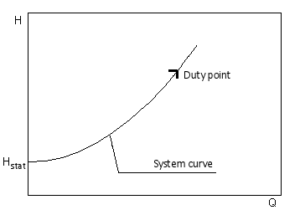
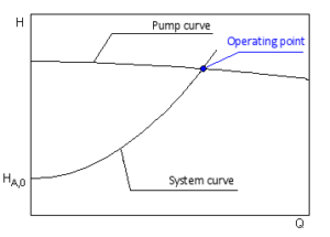
Under the above stated premises the parabolic system H-Q curve can now be drawn:
g = gravity (9.81 m/s2)
Hl,tot = total friction loss between inlet and outlet areas
vi = mean flow velocities trough pipe cross-section area
Ai = characteristic pipe cross-sectional area
ζi = friction loss coefficient for pipes, fittings, etc.
Q = flow rate
k = proportionality factor
Under the above stated premises the parabolic system H-Q curve can now be drawn:
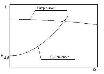
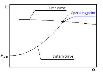
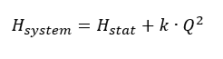 The proportionality factor k is determined of the specified duty point. The intersection of the system H-Q and the pump H-Q curves defines the actual operating point.