
 Qww – wastewater discharge (calculated flow)
K – discharge coefficient
DU – connection value of unit
Qtot – total wastewater discharge
Qs – continous wastewater discharge (without simultaneity reduction)From the sum DU, the wastewater discharge Qww can be calculated with the above formula, taking into account the corresponding discharge coefficient K. If the determined wastewater discharge Qww is smaller than the largest connected value of a single drainage object, the latter is decisive (limit value).
Qww – wastewater discharge (calculated flow)
K – discharge coefficient
DU – connection value of unit
Qtot – total wastewater discharge
Qs – continous wastewater discharge (without simultaneity reduction)From the sum DU, the wastewater discharge Qww can be calculated with the above formula, taking into account the corresponding discharge coefficient K. If the determined wastewater discharge Qww is smaller than the largest connected value of a single drainage object, the latter is decisive (limit value).Month: December 2020
Schubert & Salzer Control Systems GmbH
Waste water drainage
The wastewater discharge Qww according to DIN EN 12056-2, is determined from the sum of the connected loads (DU), taking into account the simultaneity, where K is the guide value for the discharge coefficient. It depends on the type of building and results from the frequency of use of the drainage objects. Qww – wastewater discharge (calculated flow)
K – discharge coefficient
DU – connection value of unit
Qtot – total wastewater discharge
Qs – continous wastewater discharge (without simultaneity reduction)From the sum DU, the wastewater discharge Qww can be calculated with the above formula, taking into account the corresponding discharge coefficient K. If the determined wastewater discharge Qww is smaller than the largest connected value of a single drainage object, the latter is decisive (limit value).
Qww – wastewater discharge (calculated flow)
K – discharge coefficient
DU – connection value of unit
Qtot – total wastewater discharge
Qs – continous wastewater discharge (without simultaneity reduction)From the sum DU, the wastewater discharge Qww can be calculated with the above formula, taking into account the corresponding discharge coefficient K. If the determined wastewater discharge Qww is smaller than the largest connected value of a single drainage object, the latter is decisive (limit value).Rainwater drainage
r5/2 Five-minute rainfall, which statistically must be expected once in 2 years r5/100 Five-minute rainfall, which statistically must be expected once in 100 years
DIN 1986-100 lists the values for several German cities as examples. The values differ from r5/2 =200 to 250 l/(s ha) or r5/100 = 800 l/(s ha) [1 ha = 10,000 m²].Information on rain events is available from the local authorities or alternatively from the German weather service. Reference values are given in DIN EN 1986-100 Annex A.If no values are available, rT(n)=200 l/(s ha)should be assumed. For economic reasons and in order to ensure the self-cleaning capability, pipe systems and the associated components of the rainwater drainage system shall be dimensioned for a mean rainfall event.In the scope of DIN 1986-100, the calculated rain is an idealized rain event (block rain) with a constant rain intensity over 5 minutes. The annuality (Tn) to be used for each design case is determined by the task definition. Rainfall events above the calculated rainfall (r5/2) are to be expected as planned. Qs – Rainwater drainage (calculated flow)rT(n) – Dimensioning value according to statistical eventsC – Characteristic coefficient for type of drainage areaA – Size of drainage area
Pumped medium in wastewater technology
During dimensioning, care must be taken to ensure that explosion-proof units are used to convey sewage containing faeces from shafts connected to the public sewer system.See for example also UVV 54.Kanalisationswerke:
§2 The sewer system, its access points, wells, shafts and rainwater inlets as well as collection points and venting valves in the pressure pipe system are considered to be potentially explosive in their entirety …
resp. explosion protection guidelines (Ex-RL) of the professional association (GUV 19.8) edition 06.96, example collection no. 7.3.1.1.There are, however, other regulations that may have to be taken into account. You can obtain more detailed information for your specific case from the trade association, the trade supervisory authority, the TÜV or the building authority.
Speed – Affinity Laws
The following applies:1. Model law
 2. Model law
 3. Model law
 Q – flow rate
H – delivery head
P – power consumption
n – speed
The indices relate to the respective speed.The affinity laws apply exactly to frictionless, incompressible flows. For technical applications, they are to be regarded as an approximate solution.In general, these affinity laws are independent of how the speed change is technically implemented. Traditionally, multi-speed functions of small and medium size pumps are realized by changing the motor windings configurations to achieve stepped speed variations. Meanwhile, these have been largely replaced by frequency converters.Slow-running electric drives are very expensive for larger centrifugal pumps, so that reduction gears are used for these cases.Combustion engines are used for some mobile applications. They are also variable in speed within a specified range.
Q – flow rate
H – delivery head
P – power consumption
n – speed
The indices relate to the respective speed.The affinity laws apply exactly to frictionless, incompressible flows. For technical applications, they are to be regarded as an approximate solution.In general, these affinity laws are independent of how the speed change is technically implemented. Traditionally, multi-speed functions of small and medium size pumps are realized by changing the motor windings configurations to achieve stepped speed variations. Meanwhile, these have been largely replaced by frequency converters.Slow-running electric drives are very expensive for larger centrifugal pumps, so that reduction gears are used for these cases.Combustion engines are used for some mobile applications. They are also variable in speed within a specified range.
3. Model lawQ – flow rate
H – delivery head
P – power consumption
n – speed
The indices relate to the respective speed.The affinity laws apply exactly to frictionless, incompressible flows. For technical applications, they are to be regarded as an approximate solution.In general, these affinity laws are independent of how the speed change is technically implemented. Traditionally, multi-speed functions of small and medium size pumps are realized by changing the motor windings configurations to achieve stepped speed variations. Meanwhile, these have been largely replaced by frequency converters.Slow-running electric drives are very expensive for larger centrifugal pumps, so that reduction gears are used for these cases.Combustion engines are used for some mobile applications. They are also variable in speed within a specified range.Pump Performance Curve
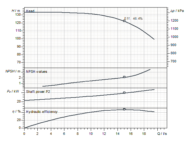
The graph of the curve is shown dropping from top left to bottom right with increasing rate of flow. The slope of the curve is determined by the pump construction and particularly by the design of the impeller.The characteristics of the pump duty curve is the inter-dependent relationship between capacity and head.Each change of head effects a consequential variation in the rate of flow.High rate of flow -> low head
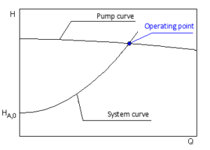
Low rate of flow -> high headThough it is the frictional resistance of the installed pipe system which determines a given pump capacity, the respective pump can take up only one duty point on its curve. This duty point is the intersection of pump H-Q curve with the system H-Q curve. In addition to the Q-H performance curve, the following performance curves are often found for centrifugal pumps:
 In addition to the Q-H performance curve, the following performance curves are often found for centrifugal pumps:
- Power
- Shaft power P2(Q)
- Electrical power consumption P1(Q)
- Efficiency
- Hydraulic efficiency ηhydr(Q)
- Total efficiency ηtot(Q)
- NPSH required NPSHreq(Q)
- Speed n(Q)
Pump Performance Chart
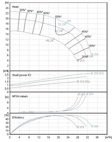
The performance curves differ in exact one parameter, such as
- Impeller diameter
- Propeller degree
- Speed
- Number of stages
Curve Corrections for Different Fluids
In practice this will however become not applicable for fluids of kinematic viscosities above 20mm²/s ( 20 cst ) due to the influence of a higher Reynolds Number with increasing viscosity. Empirical conversion methods have been developed for curve corrections for medium- and high-viscous fluids, which in practical application in older versions meant the time-consuming evaluation of diagrams, but in the current versions were prepared by corresponding formula sets.The most widespread method worldwide is the method from the Hydraulic Institute (USA), which has been standardised as ANSI/HI 9.6.7 and ISO/TR 17766. In practice, the conversion is usually carried out by computer programmes such as the Spaix PumpSelector. The computer implementation of this method enables the conversion of performance curves, whereby the user only has to define the desired delivery data and the pumped medium. The best efficiency point of the pump is of vital importance with all the known curve correction methods.The following conditions can be stated for the validity of this method:
- Centrifugal pumps with closed or semi-open impellers
- Kinematic viscosity in the range between 1 and 3000 mm²/s
- Flow rate at best efficiency point between 3 and 410 m³/h
- Head per stage between 6 and 130 m
- Fluid displacement by means of a centrifugal pump under normal operating conditions
- Handling of Newtonian Fluids
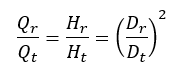
Performance curve conversion for impeller trimming
The following applies approximately: Q = flow rate
H = delivery head
D = impeller diameter
r = index for the reduced impeller diameter
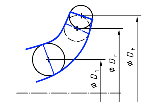
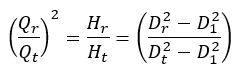
t = index for the reference wheel diameterThe throttle curve H (Q) can be roughly determined from this relationship.A more precise calculation, however, requires the consideration of performance charts in which an impeller diameter is assigned to each performance curve. The new performance curve is determined by interpolating the conversion from the neighboring curves. In order to fully utilize the efficiency of the method, it is recommended to record an duty chart with at least three performance curves. If there is a large difference between the smallest and largest impeller diameter, some (2..4) intermediate curves are required.An alternative calculation method is described in ISO 9906. Knowledge of the mean impeller diameter at the leading edge D 1 is required here. According to the standard, this procedure is valid for
Q = flow rate
H = delivery head
D = impeller diameter
r = index for the reduced impeller diameter
t = index for the reference wheel diameterThe throttle curve H (Q) can be roughly determined from this relationship.A more precise calculation, however, requires the consideration of performance charts in which an impeller diameter is assigned to each performance curve. The new performance curve is determined by interpolating the conversion from the neighboring curves. In order to fully utilize the efficiency of the method, it is recommended to record an duty chart with at least three performance curves. If there is a large difference between the smallest and largest impeller diameter, some (2..4) intermediate curves are required.An alternative calculation method is described in ISO 9906. Knowledge of the mean impeller diameter at the leading edge D 1 is required here. According to the standard, this procedure is valid for D 1 = Mean diameter at the impeller leading edgeFor pumps with a type number K ≤ 1.0 and a maximum impeller diameter reduction of 3%, the efficiency can be considered as unaltered.
 Q = flow rate
H = delivery head
D = impeller diameter
r = index for the reduced impeller diameter
t = index for the reference wheel diameterThe throttle curve H (Q) can be roughly determined from this relationship.A more precise calculation, however, requires the consideration of performance charts in which an impeller diameter is assigned to each performance curve. The new performance curve is determined by interpolating the conversion from the neighboring curves. In order to fully utilize the efficiency of the method, it is recommended to record an duty chart with at least three performance curves. If there is a large difference between the smallest and largest impeller diameter, some (2..4) intermediate curves are required.An alternative calculation method is described in ISO 9906. Knowledge of the mean impeller diameter at the leading edge D 1 is required here. According to the standard, this procedure is valid for
Q = flow rate
H = delivery head
D = impeller diameter
r = index for the reduced impeller diameter
t = index for the reference wheel diameterThe throttle curve H (Q) can be roughly determined from this relationship.A more precise calculation, however, requires the consideration of performance charts in which an impeller diameter is assigned to each performance curve. The new performance curve is determined by interpolating the conversion from the neighboring curves. In order to fully utilize the efficiency of the method, it is recommended to record an duty chart with at least three performance curves. If there is a large difference between the smallest and largest impeller diameter, some (2..4) intermediate curves are required.An alternative calculation method is described in ISO 9906. Knowledge of the mean impeller diameter at the leading edge D 1 is required here. According to the standard, this procedure is valid for- Diameter reduction up to max. 5%
- Type number K ≤ 1.5
- Unchanged blade geometry (outlet angle, tapering, etc.) after cutting
 D 1 = Mean diameter at the impeller leading edgeFor pumps with a type number K ≤ 1.0 and a maximum impeller diameter reduction of 3%, the efficiency can be considered as unaltered.