Technical Article: Energy Saving Potential for Mixing of Horizontal Flow Systems

In the water sector as well as in many other industrial sectors, there is a concern about the energy use and emission of greenhouse gasses due to climate changes. The Danish water sector branch organisation, DANVA has a vision this sector should become CO2 neutral before 2025. Already in 2007 they setup a target for 2013 stating that the water sector should reduce the energy consumption by 25% /1, 2/. The water sector uses in all around 2,4% of the total electric energy consumed in Denmark which corresponds to around 800 GWh and a resulting CO2 emission of around 470000 ton CO2/year /3/.

Of the intended savings in the water sector most should be found within wastewater treatment as this consumes around 65% of the total energy used in this sector in Denmark /4/. This figure is equal to what has been reported for the energy use of wastewater treatment plants in Massachusetts /5/. This corresponds to approximately 1% of the total amount of electric energy used in Denmark per year, where similar amounts of around 1% and 1.5% has been reported for Germany and the US respectively /6, 7, 8/.

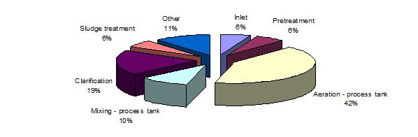
Figure 1│ Energy consumption at a wastewater treatment plant distributed on processes. Based on data from 6 Danish plants using the activated sludge process /9/.

In some cases it will be possible with simple measures to save as much as 50% of the energy just by replacing existing small diameter medium speed mixers with large diameter slow speed mixers. This will be revealed in the following study of a Danish wastewater treatment plant.

Facts about Drøsbro

Drøsbro is a small wastewater treatment plant located in Denmark. It is a biological plant with both nitrogen and phosphorous removal, but without other kinds of sludge treatment than pre-dewatering. The plant consists of a single process line with a total capacity of 10,000 PE. Of this capacity around 7,000 PE is currently used with the 388,395 m3 of wastewater treated in year 2010. The wastewater treatment plant uses 274,426 kWh per year which corresponds to 0.7 kWh/m3 or approximately 39 kWh/PE /10/. All process zones are equipped with medium speed Grundfos AMG mixers that ensure that solids are kept in suspension. The central SCADA system controls the 4 Grundfos AMG mixers with a timer controlled operation schedule of 20 minutes working time followed by 5 minutes of pause. For this work, it is only the mixer in the aerobic tank that has been studied further.

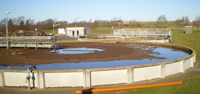
Figure 2│ The biological process tank at Drøsbro is constructed as an annular shaped tank. Inflow to the tank takes place in the innermost ring to the anaerobic zone. From here the wastewater flows to the anoxic zone via an overflow weir before it via another overflow weir enters the aerobic zone in the outermost ring. Recirculation between the aerobic and anoxic zones is handled with a horizontal low head propeller pump.

Mixing in the process tank of Drøsbro

The aerobic zone in the process tank at Drøsbro is designed to have a constant circulating flow. For mixing in these kinds of tanks basically two types of equipment can be used:

- Mixers with medium rotational speed and a small propeller diameter (AMG)

- Flowmakers with low rotational speed and a large propeller diameter (AFG)

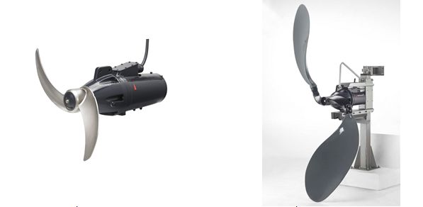
Figure 3 (Left)│Grundfos AMG mixer / Figure 4 (Right)│Grundfos AFG flowmaker

It is investigated how increasing the propeller diameter and lowering the rotational speed will influence the flow field. To make this comparison, two different two-bladed flowmakers were chosen. The rotational speed of the two flowmakers was adjusted to provide approximately the same mass flow rate as for the mixer.

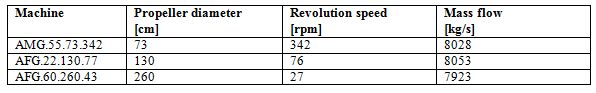
Table 1│Technical data of mixers and flowmakers

The CFD simulations

Using CFD we can build a computational model that represents a system that we want to study. The general equations for fluid flow, the Navier Stokes equations are solved and the flow field and related physical phenomena can be revealed.

Subsequently, we can analyse the results and see what impacts there are from changing the operation conditions and agitation method. In general, CFD gives us the possibility to simulate turbulent fluid flow, multiphase flows, heat and mass transfer, chemical reactions, acoustics and fluid-structure interaction. The commercial CFD software package ANSYS CFX has been used for this study.

In this case the setup of the CFD modelling has been done applying best practice guidelines developed at Grundfos over the last 5-10 years. This involves generating appropriate computational grids as well as using relevant physical models.

The tank at Drøsbro wastewater treatment plant is built of pre-fabricated concrete elements from Perstrup Beton Industri A/S and the 3D model is constructed based on appropriate detail drawings of these elements and with an applied equivalent sand roughness of 0.3 mm for the elements.

During operation of the process tank two different flow conditions can be considered. One is where the fluid is just agitated in the tank and the other one is where compressed air is added to the fluid through rows of diffuser discs at the bottom. In the first case the flow conditions will develop into a steady state open channel flow. However as is evident that in open channels smaller fluctuations in the flow field will occur but the overall flow will be more or less uniform over time. A steady state CFD simulation, which has been used in this study, will therefore capture the overall picture of the flow field and the result will resemble the general flow conditions found in the tank.

In the other case where air is supplied through the diffuser fields the flow will be heavily dominated by this and the flow has to be considered as fully transient. Comparing the flow fields in this case can only be captured by transient CFD simulations which will not be treated in this paper.

For the steady state simulations a SST turbulence model has been utilized to capture the turbulent diffusion of the flow. As it is calculation intensive and difficult to describe actual wastewater as a two phase medium of water with solids in the CFD simulation, a one phase fluid with the basic parameters of water following the non-Newtonian viscosity model of Ostwald-de Waele was chosen.

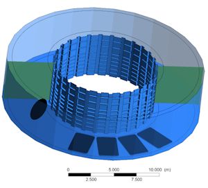
Figure 5│ The 3D model of the aerobic tank used for CFD analysis. The green planes show where cross sections for further analysis has been visualised. The black disc shows where the mixer is placed and the black rectangles indicate diffuser fields.

For each of the simulations performed a horizontal velocity contour plot in a position 0.3 m over the tank bottom plate has been visualised together with two vertical cross sections of the raceway. One cross section is placed before the mixer (left) and another is placed after the air field (right) (see 3D model for positions). For visualising the difference in propeller diameter between the three machines, the propellers have been highlighted with black on the CFD simulations.

Depending on the proceeding primary treatment it is accepted practice to keep an average velocity between 0.2-0.3 m/s over the bottom plate of the tank as an indirect measure of when suspended solids in the tank will not settle.

The flow velocity magnitudes have been visualised based on the colour bar, where velocities above 0.3 m/s are coloured with red.

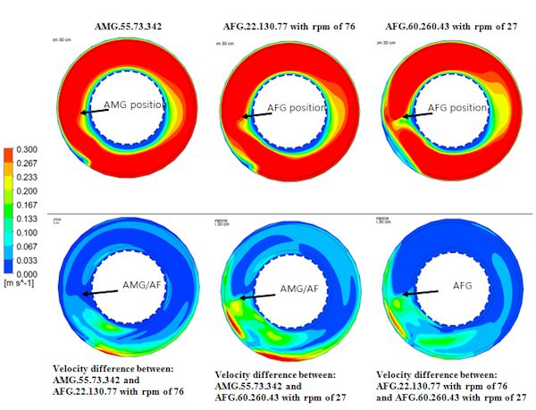
Figure 6│Velocity contour flow fields 0.3 m above the bottom of the tank.

When comparing the results of the three different machines having a similar mass flow we observe a more or less equal flow field with only smaller variations 0.3 meters above the bottom plate. As expected the velocity will be lower at the centre of the tank due to the centrifugal forces of the circulating water.

Low velocity zones shaded in blue are located in approximately the same positions and having almost the same areas and magnitudes as are high velocity zones marked with orange and red for the three different machines.

Only the AFG.60.260.43 deviates a bit from this picture as can be seen when the velocity differences are visualised. However this deviation might be due to the fact that the mass flow of the AFG.60.260.43 is around 1.5% lower compared to the two other machines in this study.

However when looking at the bulk flow in the tank judged by the cross sections below, it seems that at the right cross sections, the low velocity zone coloured in blue towards the centre of the tank is reduced as the propeller diameter is increased, which is further supported when looking at the plot of the velocity differences. At the cross sections to left there are on the contrary only minor differences in the flow fields between the three different machines. However the AFG.60.260.43 again deviates a bit from the velocity fields of the two other machines.

Figure 7│ Velocity contour flow in two different vertical cross sections of the tank.

Based on the CFD analysis doubling propeller diameter, keeping an equal mass flow, does therefore have neither a significantly positive nor a negative effect on the flow field. As the flow fields are approximately equal, independent of the propeller diameter, and thus the possibility and position of sedimentation in all three cases will possible be the same.

The determining factor for which equipment to install in the tank should purely be based on lifecycle cost of the machine or accumulated cost over a given period of time.

Savings and Lifecycle cost evaluation

Above velocity flow fields of the AFG.22.130.77 was based on an adjusted revolution speed of 76 rpm in contrary to the nominal rpm of 77. For the following calculations, data corresponding to nominal speed of the AFG.22.130.77 has been used, which to a small extend will favour the AMG.55.73.342 in below comparison as the energy consumption at 77 rpm is marginal higher that at 76 rpm.

To estimate the saving potential, the line power, P1, according to the data sheets of the products are used for the calculations when possible /11/. Here it is evident that the AMG.55.73.342 uses 5.7 kW and that the AFG.22.130.77 uses 2.5 kW during operation.

For the AFG.60.260.43 with adjusted rotational speed, it is not possible to read out P1 directly from the product data sheet. But as the efficiency is almost steady in the allowed operating range between 30-50 Hz and the turn down to 27 rpm corresponds to a frequency of 31.5 Hz, P1 for the adjusted AFG.60.260.43 can be calculated using the affinity laws.

where P is the power uptake and n is the rotational speed

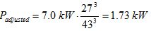
The power uptake of the AFG.60.260.43 adjusted to have a rotational speed of 27 rpm is thus 1.73 kW during operation.

Based on above power uptakes and the current operation schedule, the use of the AMG mixer in the aerobic zone of the tank consumes around 14.6% of the total energy at the plant. If in contrary an AFG.22.130.77 was installed, mixing in the aerobic zone will only consume around 7% of the total energy at the plant whereas installation of an AFG.60.260.43 with reduced revolution speed will reduce this even further to around 4.8%.

Besides the energy and thus the capital that is being saved by installing one of the AFG slow speed flowmakers compared to the current installed AMG medium speed mixer, the emission of CO2 corresponding to 0.55 kg CO2/kWh (based on Danish conditions) will also be a saved.

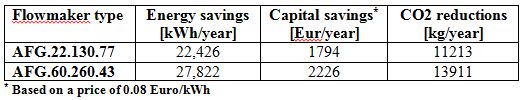
Table 2│Obtainable savings and reductions pr. year.

Without having performed a thorough CFD analysis of the anoxic process zone at Drøsbro, which also has an unrestricted circular flow, it can be speculated whether a 50% reduction in energy also can be achieved here, thus reducing the overall energy consumption even more.

Payback time for replacement of an AMG with an AFG

When calculating the payback time for replacing the AMG with one of the AFG’s it is besides the price of the specific equipment, price of energy and cost of capital also necessary to account for the cost of additional needed installation accessories, cost of a frequency converter as well as cost of the actual installation/replacement.

With a price for electricity of 0.08 Euro/kWh having an assumed steady increase of energy prices of 5% per year and a rate of interest of 5% the calculated payback times are shown in below table.

Table 3│ Calculated payback time for replacing an AMG with one of above AFG’s

With an expected lifetime for the flowmakers of 20-25 years the savings implemented by changing to an AFG.22.130.77 will contribute positively on the accounts plenty of years after the payback time which makes this investment quit attractive. With the AFG.60.260.43 a further energy saving can be achieved but the payback time is not as attractive when the alternative with the AFG.22.130.77 exists. This is due to the fact that only part of the capacity of the machine is utilised and the energy savings are not sufficient to compensate for the higher cost of the flowmaker itself, the price of the frequency converter as well as the need for more sturdy installation accessories compared to what is needed for the AFG.22.130.77.

Payback time for installing an AFG compared to an AMG

For new installations and upgrade projects it is another situation. A comparison has been made by looking at the accumulated cost per month (figure 8), thus the initial cost of equipment and installation accessories plus the operational cost, where the energy prices are expected to increase with 5% pr. year.

From this calculation it can be observed that significant savings can be achieved by installing an AFG.22.130.77 compared to the AMG.55.73.342. In less than 12 months, the higher investment of the AFG.22.130.77 will be justified due to the lower energy consumption during operation.

Even with the investment and need for a frequency converter the payback time of the AFG.66.260.43, will in this case only be around 44 months.

However considering the radial flow that will arrive at the propeller, due to the circular tank shape and the resulting flow velocity gradient that arise over the propeller, it makes a flowmaker with a diameter of 2.6 meter a less attractive alternative than a flowmaker with a diameter of 1.3 meter as there is no extra improvement in the flow velocity distribution in the tank.

Figure 8│ Accumulated cost as a function of time.

Conclusions

Based on analysis of velocity flow fields using Computational Fluid Dynamics it has been shown that for Drøsbro wastewater treatment plant a replacement of the AMG.55.73.342 to an AFG.22.130.77 in the aerobic zone can reduce the total energy used for mixing at the plant from 14.5 % to 7 % without altering the flow field and thus the mixing of the tank. The payback time for implementing this exchange of equipment in the aerobic zone of the plant will be around 4 years. For Drøsbro this will lower the key performance figures from 39 kWh/PE to 36 kWh/PE. Furthermore it will reduce the emission of CO2 with around 11,200 kg/year which minimises the burden on the environment.

Based on findings in this study, process tanks with unrestricted flow could potential find easy and economical justified energy savings by using low speed large diameter propeller flowmakers compared to medium speed small diameter propeller mixers despite the higher initial cost of a flowmaker.

Acknowledgements

The author would like to thank Favrskov Forsyning for granting access to Drøsbro wastewater treatment plant as a vital part of this work.

Author

Bruno Kiilerich, Application specialist, Water Utility

Eddy Yang, Development Engineer, Structural Fluid Mechanics

Grundfos Management, Poul Due Jensens Vej 7, 8850 Bjerringbro

References

/1/ “Inspirationsguide for proaktiv klimatilpasning i vandsektoren”, DANVA and KL, Oktober 2009, ISBN 87-90455-91-6

/2/ “http://www.danva.dk/Default.aspx?ID=2241&TokenExist=no”, DANVA

/3/ “Drivhusgasser skal reducers med en faktor 10”, danskVand, volume 76, no. 5, August 2008

/4/ “Vurdering af energibesparelsespotentialet i vandsektoren” Elspare Fonden prepared by Jan Egelund Grontmij | Carl Bro, May 2007

/5/ “Ensurering a sustainable future - and energy management guidebook for wastewater and water utilities” EPA, January 2008

/6/ “Elbesparelse ved integreret optimering af processer og bundbeluftning i kommunale og industrielle renseanlæg”, Energistyrelsen, ENS Journalnr. 127-0031 prepared by DHI, 2003

/7/ “Municipal wastewater treatment plant energy baseline study”, PG&E new construction energy management program, prepared by M/J Industrial Solutions San Francisci, CA 94122, June 2003

/8/ “Steigerung der Energieeffizienz auf kommunalen Kläranlagen”, Umwelt Bundes Amt, Texte 11 | 8, 2008, ISSN 1862-4804

/9/ http://www.energibesparelser-vand.dk/Default.aspx?ID=1249&TokenExist=no, DANVA

/10/ “Grønt regnskab for offentlige renseanlæg 2010”, Favrskov Forsyning A/S

/11/ “Grundfos Data Booklet, Mixers and Flowmakers, AMD, AMG, AFG, 50 Hz”, Grundfos